Fractal Dimension Reduction for Topic Modeling
In this post, I will share an alternative approach to mine important topics from Data Science Blog headlines. This approach does not use clustering, but tries to explain document embeddings along interpretable dimensions. Many reprojections using PCA and the likes are possible. We want to use an approximation of the datasets intrinsic dimensions, the fractal dimension of the reprojection method. Fractal dimension measures how simple (low) or complex (high) a dataset really is. We approximate the true form of the data via reprojection by rounding from the number of fractal dimensions of the data.
We can use word embedding to create a semantic representation of documents and phrases. Common approaches then apply clustering algorithms to extract topics. I’ve made good experiences with hierarchical clustering and mid sized clusters. Nonetheless, I have been dissatisfied by the fact this approach leaves the user to decide what topic to learn about first. The size of the clusters is not always a good representation how important it really is for the discourse at hand, especially if the data does not center around clearly separable classes.
An alternative approach I came to like is to use dimension reduction, namely PCA and factor loadings to find topic loaded keywords, which explain most of the variance in the data. On informal tests with clearly separated data, PCA put the data on some of the classes as dimensions.
However, PCA yields a lot of dimensions.
The motivation for this experiment is twofold:
- Find the true number of reduced dimensions in the data by observing at which number of retained dimensions the fractal dimension of the dataset stabilizes.
- Try out non-linear dimension reduction with an autoencoder, apply predictive power score to find labels for the dimensions and compare its fractal dimension with the PCAs results. Check if the method with more fractal dimensions yields better dimensions, as suggested in the literature (see https://www.ml.cmu.edu/research/dap-papers/skkumar_kdd_project.pdf).
Ideally this should yield a low number of dimensions, which help us to quickly understand core thoughtgood. The dimensions can be used to plot and analyse the data, directly or to guide at which topics (by their keyword labels) to look first using conventional embedding based methods.
Fractal PCA
Let’s see how many intrinsic dimensions different PCA solutions have. I choose a method which estimates intrinsic dimensions relatively fast, for practical reasons.
In the plot we see, the number only slowly increases beyond 10 intrinsic dimensions. The fractal dimension with the first 100 is below 12.85. 12 intrinsic dimensions are reasonable.
pacman::p_load(tidyverse, tidytable, data.table, tidytext, textrank, job, UBL, archetypes, future, future.callr, genieclust, doc2vec, quanteda, udpipe, qrpca, ider, ranger, ggcorrplot)


blogposts <- fread("/home/knut/Desktop/my_niche/data/twds_scrape_distinct.csv")

titles <- blogposts %>% filter.(variable=="title") %>% distinct(value)

f <- callr({
  library(reticulate)
  use_python("/home/knut/transformers/bin/python", required = T)
  st <- import("sentence_transformers")
  model <- st$SentenceTransformer('all-mpnet-base-v2')
  embeddings = model$encode(titles$value)

}, workers=1)


embeddings <- value(f)


# extract descriptive keywords

f <- callr({
  library(spacyr)
  spacy_initialize(model = "en_core_web_trf", python_executable = "/home/knut/transformers/bin/python3")

  tags <- spacy_parse(titles$value)


}, workers=1)


tags <- value(f)

title_tags <- tags %>% mutate(id=stringr::str_remove(doc_id, "text") %>% as.numeric()) %>% inner_join.(titles %>% mutate(id=row_number()))


keyw <- textrank_keywords(title_tags$lemma,
                          relevant = title_tags$pos %in% c("NOUN", "VERB", "ADJ"), p = 0.3)
keyw <- subset(keyw$keywords, ngram > 0 & freq > 1)%>% mutate(title=str_replace_all(keyword, "-", " "))

keyw$title <- str_squish(keyw$title)


titles_ngrams <- titles %>% unnest_ngrams(output = "ngram", input = "value", n = 3, n_min = 1, drop = F) %>% inner_join.(keyw %>% mutate(ngram=title))


titles_ngrams <- titles_ngrams %>% inner_join.(titles %>% distinct.(value) %>% mutate(doc_id=row_number()))

x <- document_term_frequencies(titles_ngrams[, c("doc_id", "ngram")])

dfm <- document_term_matrix(x) %>% as.dfm() %>% as.matrix() %>% data.table::as.data.table() %>% mutate(value=titles_ngrams$value %>% unique())%>% imputeTS::na.replace(0)


#pca

embeddings_filtered <- embeddings[titles %>% mutate(doc_id=row_number()) %>% filter.(value%in%titles_ngrams$value) %>% pull(doc_id),]


pca1 <- qrpca(embeddings_filtered)

loadings <- pca1$rotation %>% as.data.frame()


components <- pca1$x %>% as.data.frame()

#estimate fractal dims

fractal_dims <- data.table(dim=c(), fractal_dim=c())

for (i in 5:30){
  components_part <- components[,1:i]
  fractal_dimension <- nni(components_part)
  fractal_dims <- fractal_dims %>% bind_rows.(data.table(dim=i, fractal_dim=fractal_dimension))
  print(c(i, fractal_dimension))
}
## [1] 5.000000 4.897236
## [1] 6.000000 5.666823
## [1] 7.000000 6.322528
## [1] 8.000000 6.879264
## [1] 9.000000 7.382553
## [1] 10.000000 7.827464
## [1] 11.000000 8.181225
## [1] 12.000000 8.484103
## [1] 13.000000 8.749288
## [1] 14.000000 9.016126
## [1] 15.000000 9.265952
## [1] 16.000000 9.420807
## [1] 17.000000 9.634053
## [1] 18.000000 9.788483
## [1] 19.0000 9.9498
## [1] 20.00000 10.06284
## [1] 21.00000 10.22702
## [1] 22.00000 10.34785
## [1] 23.00000 10.41959
## [1] 24.00000 10.51443
## [1] 25.00000 10.59699
## [1] 26.00000 10.68032
## [1] 27.00000 10.75729
## [1] 28.00000 10.83393
## [1] 29.00000 10.90076
## [1] 30.00000 10.96492ggplot(fractal_dims) +
aes(x = dim, y = fractal_dim) +
geom_line(size = 0.5, colour = "#112446") +
theme_minimal()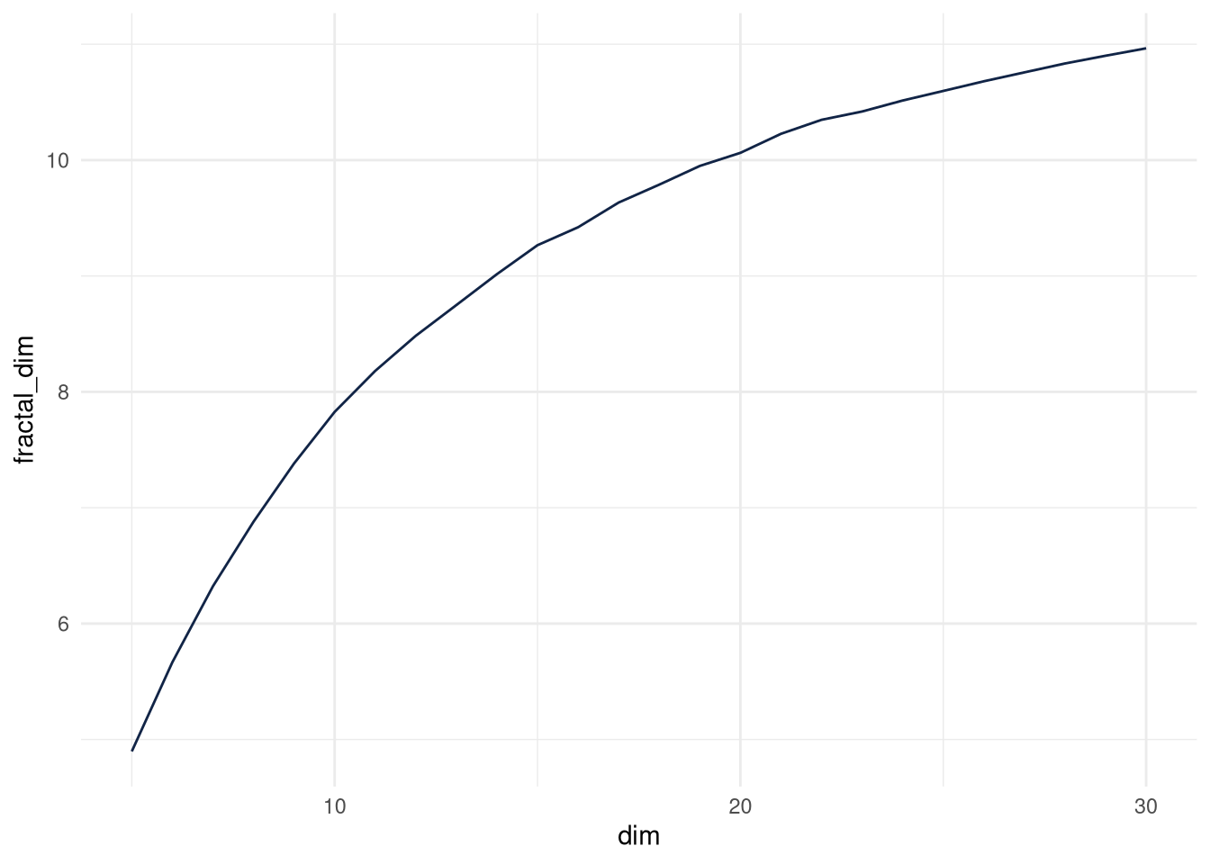
What keywords are associated with fractal principal components?
Deep learning, python, coding, databases, nlp, deployment, ML, introductions, algorithms, data science and visualisation seem to organize the headlines.
components_part <- components[,1:12]

correlation_matrix <- cor(dfm %>% select(-value) %>% as.matrix(), components_part)
rotatedLoadings <- varimax(correlation_matrix)
l <- rotatedLoadings$loadings
rotatedLoadings <- data.frame(matrix(as.numeric(l), attributes(l)$dim, dimnames=attributes(l)$dimnames))


rotatedLoadings$token <- rownames(rotatedLoadings)
rotatedLoadings <- rotatedLoadings %>% filter(token%in%colnames(embeddings %>% as.data.frame)==F) %>% data.table::melt(id.vars="token")
rotatedLoadings <- rotatedLoadings %>% group_by(variable) %>% arrange(desc(value),.by_group = T) %>% top_n.(10, .by = variable)

ggcharts::bar_chart(rotatedLoadings, x = token, y = value, facet = variable, top_n = 15)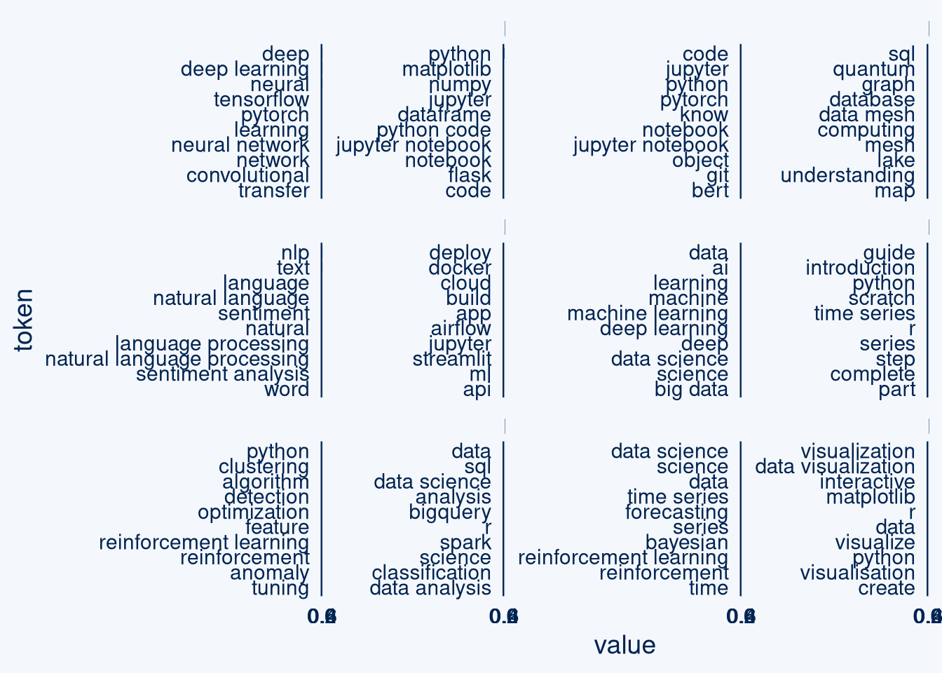
Fractal Autoencoder
For the autoencoder, I initially trained one with 100 latent dimensions. It had 13.44 intrinsic dimensions. Looping shows intrinsic dimension flattens out with 10 intrinsic dimensions, I grab 12.
fractal_dims <- data.table(dim=c(), fractal_dim=c())

# for (i in 5:30){
#   f <- callr({
#     library(reticulate)
#     use_python("/home/knut/cvae/bin/python", required = T)
#     cvae <- import("cvae")$cvae
#     embedder <- cvae$CompressionVAE(embeddings, dim_latent=as.integer(i))
#     embedder$train()
#     CompressionVAE <- embedder$embed(embeddings)
#
#   }, workers=1)
#
#
#   CompressionVAE <- value(f)
#   fractal_dimension <- nni(CompressionVAE)
#   fractal_dims <- fractal_dims %>% bind_rows.(data.table(dim=i, fractal_dim=fractal_dimension))
#   print(c(i, fractal_dimension))
# }


ggplot(fread("/home/knut/Desktop/fractal_dims_autoenc.csv")) +
  aes(x = dim, y = fractal_dim) +
  geom_line(size = 0.5, colour = "#112446") +
  theme_minimal()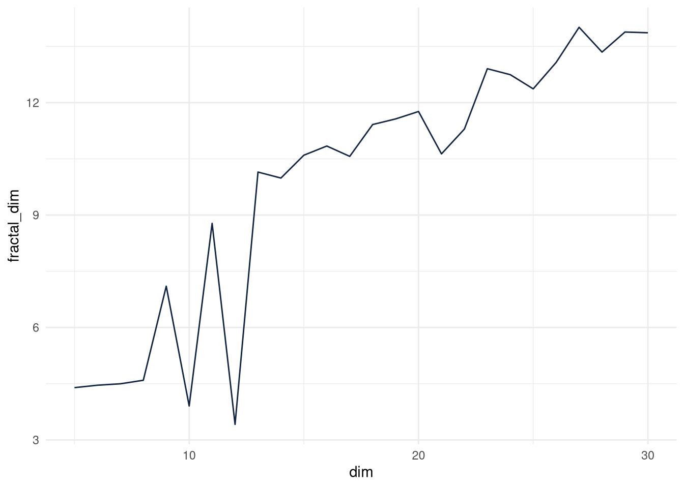
This is what a scatterplot matrix of the autoencoder looks like. These should also be a nice basis for cluster based topic modeling in a later step. We can see some nice correlations:
  # f <- callr({
  #   library(reticulate)
  #   use_python("/home/knut/cvae/bin/python", required = T)
  #   cvae <- import("cvae")$cvae
  #   embedder <- cvae$CompressionVAE(embeddings, dim_latent=as.integer(12), batch_size = 1L)
  #   embedder$train()
  #   CompressionVAE <- embedder$embed(embeddings)
  #
  # }, workers=1)
  #
  #
  # CompressionVAE <- value(f)
  # nni(CompressionVAE)


autoencoder_embeddings <- fread("/home/knut/Desktop/autoenc.csv")

GGally::ggpairs(autoencoder_embeddings)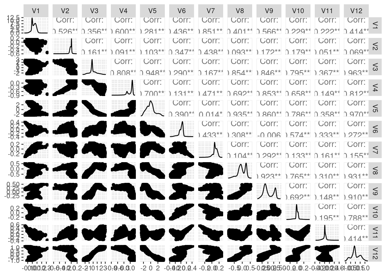
We don’t have labels for the dimensions yet and don’t know which dimensions are more important. As easy approach, I’ll just estimate variable importance of document feature matrixes of keywords predicting each autoencoder dimension for themselves.
To order dimension importance (as variance explained does so naturally for PCA), I’ll use unsupervised random forest.
Parts of this code takes some time to run, so I reload results.
These results are different from PCA, as the dimensions are not required to be orthogonal, is more overlap.
So I summarize keywords accross dimensions with a simple count and tf-idf keywords to signify differences.
Let’s first look at the general topics, which span across different dimensions. For simplicities sake I grab the top 50 most important terms and count them. The word cloud plot directly shows across how many dimensions the words were in the 50 most important keywords.
rnumbers <- titles %>% mutate(id=row_number()) %>% inner_join.(titles_ngrams %>% distinct.(value)) %>% pull(id)

# v1 <- bind_cols.(dfm, autoencoder_embeddings[rnumbers,] %>% select(V1))
# v2 <- bind_cols.(dfm, autoencoder_embeddings[rnumbers,] %>% select(V2))
# v3 <- bind_cols.(dfm, autoencoder_embeddings[rnumbers,] %>% select(V3))
# v4 <- bind_cols.(dfm, autoencoder_embeddings[rnumbers,] %>% select(V4))
# v5 <- bind_cols.(dfm, autoencoder_embeddings[rnumbers,] %>% select(V5))
# v6 <- bind_cols.(dfm, autoencoder_embeddings[rnumbers,] %>% select(V6))
# v7 <- bind_cols.(dfm, autoencoder_embeddings[rnumbers,] %>% select(V7))
# v8 <- bind_cols.(dfm, autoencoder_embeddings[rnumbers,] %>% select(V8))
# v9 <- bind_cols.(dfm, autoencoder_embeddings[rnumbers,] %>% select(V9))
# v10 <- bind_cols.(dfm, autoencoder_embeddings[rnumbers,] %>% select(V10))
# v11 <- bind_cols.(dfm, autoencoder_embeddings[rnumbers,] %>% select(V11))
# v12 <- bind_cols.(dfm, autoencoder_embeddings[rnumbers,] %>% select(V12))
#
#
#
# # dfm variable importance per latent variable
#
# v1.rg = ranger::ranger(data = v1, dependent.variable.name = "V1", importance = "impurity") %>% importance()
# v2.rg = ranger::ranger(data = v2, dependent.variable.name = "V2", importance = "impurity") %>% importance()
# v3.rg = ranger::ranger(data = v3, dependent.variable.name = "V3", importance = "impurity") %>% importance()
# v4.rg = ranger::ranger(data = v4, dependent.variable.name = "V4", importance = "impurity") %>% importance()
# v5.rg = ranger::ranger(data = v5, dependent.variable.name = "V5", importance = "impurity") %>% importance()
# v6.rg = ranger::ranger(data = v6, dependent.variable.name = "V6", importance = "impurity") %>% importance()
# v7.rg = ranger::ranger(data = v7, dependent.variable.name = "V7", importance = "impurity") %>% importance()
# v8.rg = ranger::ranger(data = v8, dependent.variable.name = "V8", importance = "impurity") %>% importance()
# v9.rg = ranger::ranger(data = v9, dependent.variable.name = "V9", importance = "impurity") %>% importance()
# v10.rg = ranger::ranger(data = v10, dependent.variable.name = "V10", importance = "impurity") %>% importance()
# v11.rg = ranger::ranger(data = v11, dependent.variable.name = "V11", importance = "impurity") %>% importance()
# v12.rg = ranger::ranger(data = v12, dependent.variable.name = "V12", importance = "impurity") %>% importance()
#
#
# #unsupervised random forest latent variable importance
#
# urf <- randomUniformForest::unsupervised.randomUniformForest(autoencoder_embeddings, ntree=1000)
# urf_supervised <- as.supervised(urf, autoencoder_embeddings, bagging=TRUE, ntree=500)
# urf_importance <- importance(urf_supervised, Xtest = autoencoder_embeddings)


fastSave::load.lbzip2("/home/knut/Desktop/unsupervised_rf.RDataFS")

general_keywords <- urf_importance$globalVariableImportance %>% left_join(data.table(importance=c(v1.rg, v2.rg, v3.rg, v4.rg, v5.rg, v6.rg, v7.rg, v8.rg, v9.rg, v10.rg, v11.rg, v12.rg), keyword=names(c(v1.rg, v2.rg, v3.rg, v4.rg, v5.rg, v6.rg, v7.rg, v8.rg, v9.rg, v10.rg, v11.rg, v12.rg)), variables=c(rep("V1", length(v1.rg)), rep("V2", length(v2.rg)), rep("V3", length(v3.rg)), rep("V4", length(v4.rg)), rep("V5", length(v5.rg)), rep("V6", length(v6.rg)), rep("V7", length(v7.rg)), rep("V8", length(v8.rg)), rep("V9", length(v9.rg)), rep("V10", length(v10.rg)), rep("V11", length(v11.rg)), rep("V12", length(v12.rg)))) %>% group_by(variables) %>% arrange(desc(importance)) %>% slice_head(n = 50)) %>% filter(keyword!="value")
general_keywords_frequencies <- general_keywords %>% group_by(keyword) %>% count(sort = T)

wordcloud2::wordcloud2(general_keywords_frequencies %>% rename(word=keyword, freq=n), size = 0.3)
General topics include data science, deep learning, machine learning, classification, neural nets, visualizations, careers.
general_keywords_frequencies ## # A tibble: 130 × 2
## # Groups: keyword [130]
## keyword n
## <chr> <int>
## 1 data 12
## 2 data science 12
## 3 deep 12
## 4 deep learning 12
## 5 learning 12
## 6 machine 12
## 7 machine learning 12
## 8 neural 12
## 9 python 12
## 10 pytorch 12
## # … with 120 more rowsSo what about dimension distinguishing important keywords?
I removed the general topics as stopwords, below we see the variable importance for terms in random forests predicting each latent variable.
These latent variables are also sorted for their unsupervised random forest importance.
It is not surprising that the general topics AI (and properly lots of general data science topics) are fractal dimension 9, which also correlates with V8 (BI jobs), V10 and V6 (learning data science), V12 (data visualization).
Covid 19 / NLP market intelligence and neural nets also seem to organize the topics.
distinctive_keywords <- general_keywords %>% filter(keyword%in%(general_keywords_frequencies %>% filter(n>4) %>% pull(keyword))==F) %>% mutate(variables=factor(variables, levels = urf_importance$globalVariableImportance %>% pull(variables)))


cowplot::plot_grid(ggcharts::bar_chart(distinctive_keywords, x = keyword, y = importance, facet = variables, top_n = 15), ggcorrplot(autoencoder_embeddings %>% cor()), ncol = 2, rel_widths = c(3,1))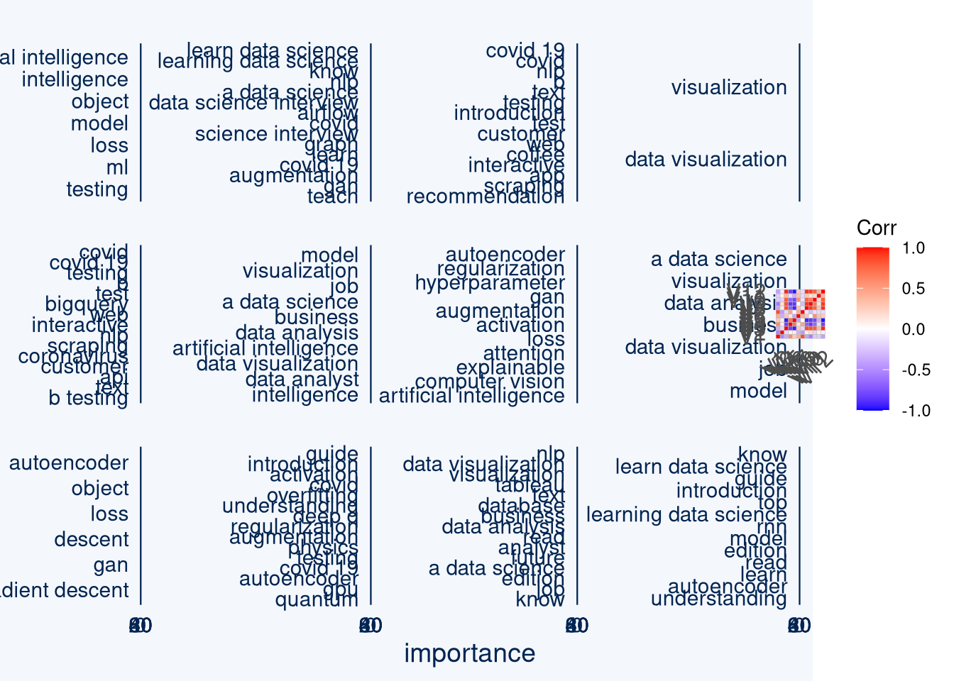
Conclusion
We can see, that using fractal dimensions to project the dataset into intrinsic, interpretable and approximately true dimensions help a lot to get a general overview on what topics are influential in those data science headlines. These topics as well as the projections are great starting points for clustering based topic modelling and weak labeling with those keywords.